Tips for spatiotemporal indexing

In the both the AdaSTEM Demo and SphereAdaSTEM demo we use bird observation data to demonstrate functionality of AdaSTEM. Spatiotemporal coordinate are homogeneously encoded in these two cases, with longitude and latitude being spatial indexes and DOY (day of year) being temporal index.

Here, we present more tips and examples on how to play with these indexing systems.

2D + Temporal indexing

Flexible coordinate systems

stemflow support all types of spatial coordinate reference system (CRS) and temporal indexing (for example, week month, year, or decades). stemflow only support tabular point data currently. You should transform your data to desired CRS before feeding them to stemflow.

For example, transforming CRS:

import pyproj

# Define the source and destination coordinate systems
source_crs = pyproj.CRS.from_epsg(4326)  # WGS 84 (latitude, longitude)
target_crs = pyproj.CRS.from_string("ESRI:54017")  # World Behrmann equal area projection (x, y)

# Create a transformer object
transformer = pyproj.Transformer.from_crs(source_crs, target_crs, always_xy=True)

# Project
data['proj_lng'], data['proj_lat'] = transformer.transform(data['lng'].values, data['lat'].values)

Now the projected spatial coordinate for each record is stored in data['proj_lng'] and data['proj_lat'] We can then feed this data to stemflow:

from stemflow.model.AdaSTEM import AdaSTEMClassifier
from xgboost import XGBClassifier

model = AdaSTEMClassifier(
    base_model=XGBClassifier(tree_method='hist',random_state=42, verbosity = 0,n_jobs=1),
    save_gridding_plot = True,
    ensemble_fold=10,                      # data are modeled 10 times, each time with jitter and rotation in Quadtree algo
    min_ensemble_required=7,               # Only points covered by > 7 stixels will be predicted
    grid_len_upper_threshold=1e5,          # force splitting if the edge of grid exceeds 1e5 meters
    grid_len_lower_threshold=1e3,          # stop splitting if the edge of grid fall short 1e3 meters             
    temporal_start=1,                      # The next 4 params define the temporal sliding window
    temporal_end=52,                            
    temporal_step=2,
    temporal_bin_interval=4,
    points_lower_threshold=50,             # Only stixels with more than 50 samples are trained
    Spatio1='proj_lng',                    # Use the column 'proj_lng' and 'proj_lat' as spatial indexes
    Spatio2='proj_lat',
    Temporal1='Week',
    use_temporal_to_train=True,            # In each stixel, whether 'Week' should be a predictor
    njobs=1
)

Here, we use temporal bin of 4 weeks and step of 2 weeks, starting from week 1 to week 52. For spatial indexing, we force the gird size to be 1km (1e3 m) ~ 10km (1e5 m). Since ESRI 54017 is an equal area projection, the unit is meter.

Then we could fit the model:

## fit
model = model.fit(data.drop('target', axis=1), data[['target']])

## predict
pred = model.predict(X_test)
pred = np.where(pred<0, 0, pred)
eval_metrics = AdaSTEM.eval_STEM_res('classification',y_test, pred_mean)

Note that the Quadtree [1] algo is limited to 6 digits for efficiency. So transform your coordinate of it exceeds that threshold. For example, x=0.0000001 and y=0.0000012 will be problematic. Consider changing them to x=100 and y=1200.

Spatial-only modeling

By playing some tricks, you can also do a spatial-only modeling, without splitting the data into temporal blocks:

model = AdaSTEMClassifier(
    base_model=XGBClassifier(tree_method='hist',random_state=42, verbosity = 0,n_jobs=1),
    save_gridding_plot = True,
    ensemble_fold=10,
    min_ensemble_required=7,
    grid_len_upper_threshold=1e5,
    grid_len_lower_threshold=1e3,
    temporal_start=1,
    temporal_end=52,                            
    temporal_step=1000,                 # Setting step and interval largely outweigh 
    temporal_bin_interval=1000,         # temporal scale of data
    points_lower_threshold=50,             
    Spatio1='proj_lng',                   
    Spatio2='proj_lat',
    Temporal1='Week',
    use_temporal_to_train=True,
    njobs=1
)

Setting temporal_step and temporal_bin_interval largely outweigh the temporal scale (1000 compared with 52) of your data will render only one temporal window during splitting. Consequently, your model would become a spatial model. This could be beneficial if temporal heterogeneity is not of interest, or without enough data to investigate.

Fix the gird size of Quadtree algorithm

There are two ways to fix the grid size:

1. By using some tricks we can fix the gird size/edge length of AdaSTEM model classes:

model = AdaSTEMClassifier(
    base_model=XGBClassifier(tree_method='hist',random_state=42, verbosity = 0,n_jobs=1),
    save_gridding_plot = True,
    ensemble_fold=10,
    min_ensemble_required=7,
    grid_len_upper_threshold=1000,
    grid_len_lower_threshold=1000,
    temporal_start=1,
    temporal_end=52,                            
    temporal_step=2,                 
    temporal_bin_interval=4,         
    points_lower_threshold=0, 
    stixel_training_size_threshold=50,            
    Spatio1='proj_lng',                   
    Spatio2='proj_lat',
    Temporal1='Week',
    use_temporal_to_train=True,
    njobs=1
)

Quadtree will keep splitting until it hits an edge length lower than 1000 meters. Data volume won't hamper this process because the splitting threshold is set to 0 (points_lower_threshold=0). Stixels with sample volume less than 50 still won't be trained (stixel_training_size_threshold=50). However, we cannot guarantee the exact grid length. It should be somewhere between 500m and 1000m since each time Quadtree do a bifurcated splitting.

2. Using `STEM` model classes

We also implemented STEM model classes for fixed gridding. Instead of adaptive splitting based on data abundance, STEM model classes split the space with fixed grid length:

from stemflow.model.STEM import STEM, STEMRegressor, STEMClassifier

model = STEMClassifier(
    base_model=XGBClassifier(tree_method='hist',random_state=42, verbosity = 0,n_jobs=1),
    save_gridding_plot = True,
    ensemble_fold=10,
    min_ensemble_required=7,
    grid_len=1000,
    temporal_start=1,
    temporal_end=52,                            
    temporal_step=2,                 
    temporal_bin_interval=4,         
    points_lower_threshold=0, 
    stixel_training_size_threshold=50,            
    Spatio1='proj_lng',                   
    Spatio2='proj_lat',
    Temporal1='Week',
    use_temporal_to_train=True,
    njobs=1
)

Here, grid_len parameter take place the original upper and lower threshold parameters. The main functionality is the same as AdaSTEM classes.

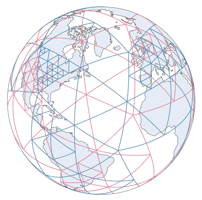
3D spherical + Temporal indexing

Our earth is a sphere, and consequently there is no single solution to project the sphere to a 2D plane while maintaining the distance and area – all projection method as pros and cons. We also implemented spherical indexing to solve this issue.

from stemflow.model.SphereAdaSTEM import SphereAdaSTEMRegressor
from xgboost import XGBClassifier, XGBRegressor

model = SphereAdaSTEMRegressor(
    base_model=Hurdle(
        classifier=XGBClassifier(tree_method='hist',random_state=42, verbosity = 0, n_jobs=1),
        regressor=XGBRegressor(tree_method='hist',random_state=42, verbosity = 0, n_jobs=1)
    ),                                # hurdel model for zero-inflated problem (e.g., count)
    save_gridding_plot = True,
    ensemble_fold=10,                 # data are modeled 10 times, each time with jitter and rotation in Quadtree algo
    min_ensemble_required=7,          # Only points covered by > 7 stixels will be predicted
    grid_len_upper_threshold=2500,    # force splitting if the grid length exceeds 2500 (km)
    grid_len_lower_threshold=500,     # stop splitting if the grid length fall short 500 (km)        
    temporal_start=1,                 # The next 4 params define the temporal sliding window
    temporal_end=366,                            
    temporal_step=25,                 # The window takes steps of 20 DOY (see AdaSTEM demo for details)
    temporal_bin_interval=50,         # Each window will contain data of 50 DOY
    points_lower_threshold=50,        # Only stixels with more than 50 samples are trained
    Temporal1='DOY',
    use_temporal_to_train=True,       # In each stixel, whether 'DOY' should be a predictor
    njobs=1
)

SphereAdaSTEM module has almost the same structure and functions as AdaSTEM and STEM modules. The only difference is that

It mandatorily looks for "longitude" and "latitude" in the columns.
It splits the data using Sphere QuadTree [2].
It plots the grids using plotly.

See SphereAdaSTEM demo and Interactive spherical gridding plot.

References:

- Samet, H. (1984). The quadtree and related hierarchical data structures. ACM Computing Surveys (CSUR), 16(2), 187-260.
- Gyorgy, F. (1990, October). Rendering and managing spherical data with sphere quadtrees. In Proceedings of the First IEEE Conference on Visualization: Visualization90 (pp. 176-186). IEEE.